Dynamics, Linear Systems and Equilibria Review#
Continuous Time Dynamics#
The dynamics of a smooth system can generally be defined as
where \(\dot{x}\) is the time derivative of the “state” \(x\in\mathbb{R}^N\). The control “input” is \(u\in\mathbb{R}^M\).
Note
The size of \(\dot{x}\) is not necessarily the same as \(x\) such as in the case of derivatives of rotations [Ted23].
For a mechanical system, the state is usually stacked positions and veclocities known as the “configuration”.
Example Pendulum#
Simple pendulum dynamics are given as:
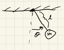
Then the pendulum can be represented as a system of first order ODEs with:
\(q\in\mathbb{S}^1\) (a circle) and \(x\in\mathbb{S}^1 \times \mathbb{R}\) (a cyclinder).
# Activate the enironment
import Pkg
Pkg.activate(@__DIR__); # activate the env in the directory
# Pkg.instantiate()
using Plots

function dynamics(params::NamedTuple, x::Vector, u)
    # pendulum ODE, parametrized by params.

    m, l, g = params.m, params.l, params.g

    θ = x[1]
    dθ= x[2]

    # return [dθ; -g/l * sin(θ) + u/(m*l^2) - dθ] # Try adding a damping term to the system
    return [dθ; -g/l * sin(θ) + u/(m*l^2)]

end

function rk4(params::NamedTuple, x::Vector, u , dt::Float64)
    # vanilla RK4
    k1 = dt*dynamics(params, x, u)
    k2 = dt*dynamics(params, x + k1/2, u)
    k3 = dt*dynamics(params, x + k2/2, u)
    k4 = dt*dynamics(params, x + k3, u)
    x + (1/6)*(k1 + 2*k2 + 2*k3 + k4)
end
Activating project at `/__w/CMU-16-745/CMU-16-745/optimalcontrol`
rk4 (generic function with 1 method)
Show code cell content
function animate_pendulum(params, t, X)
    anim = @animate for i in 1:length(t)
        x = [0; params.l * sin(X[1, i])]
        y = [0; -params.l * cos(X[1, i])]
        view = 2 * params.l
        plot(x,y, color=:blue, label="")
        plot!([x[2]], [y[2]], seriestype=:scatter, color=:blue, label="")
        plot!(xlims=(-view, view),
            ylims=(-view, view),
            aspect_ratio=:equal)
        plot!(title="t = "*string(t[i]))

    end
    gif(anim, show_msg=false)
end
animate_pendulum (generic function with 1 method)
# Define the pendulum params
params = (m=0.1,l=0.1, g=9.81)

# Preallocate
dt = 0.01
t = 0:dt:2
X = zeros(2, length(t))
X[:,1] = [π/4, 0] # initial condition
u = 0

# Simulate
for i in 1:length(t)-1
    X[:,i+1] = rk4(params, X[:,i], u , dt)
end

# Plot
plot(t, X', layout=(2,1), label=["theta" "dtheta"])
plot!(xlabel="t")
Show code cell source
animate_pendulum(params, t, X)

Control - Affine Systems#
A system is “control affine” if it can be put in the form
Most systems can be put in this form.
Manipulator Dynamics#
Where \(M\) is the mass matrix, \(C\) is the Coriolis and gravity terms, \(B\) is the input Jacobian and \(F\) are external forces.
All mechanical systems can be written like this.
It is a rearranging of the Euler-Lagrange equation
Which is the kinetic energy minus the potential energy.
Linear Systems#
The system is linear in \(x\) and \(u\) if it is of the form
It is time invariant if \(A(t) = A\) and \(B(t) = B\) (ie constant).
Nonlinear systems are often approximated with linear systems.
Equilibria#
A point where the system will “remain at rest”
Algebraically, these are the roots of the dynamics.
For example the pendulum
But in general we have a root-finding problem in \(u\). That is
First Control Example#
For the pendulum system we can introduce a control to achieve a desired set point.
This is analytic
Though this doesn’t work well, here or in practice, due to the control lagging the system state (sensor readings).
To counter this let’s use this as a feedforward controller and cancel out and disturbances with a PD term. So we will have a feedforward PD controller.
# Now what if we force it
X[:,1] = [π/4; 0.1]

# With only feedforward term, small errors cause instability (in sim, in model, unmodelled)
# Try changing the gains to zero to demonstrate this
# Note that a real system might have daming to counter this
function feedforward_pd(setpoint::Vector, X::Vector, kp, kd)
    # Cancel the velocity
    ex = setpoint[1] - X[1] # Pid term
    ev = setpoint[2] - X[2] # Velocity damping
    ff = params.m*params.g*params.l # Feed forward torque
    return kp*ex + kd*ev + ff
end

# Simualte with control
for i in 1:length(t)-1
    u = feedforward_pd([π/2; 0.0], X[:,i], 3, 0.05)
    X[:,i+1] = rk4(params, X[:,i], u , dt)
end

# Plot
plot(t, X', layout=(2,1), label=["theta" "dtheta"]);
plot!(xlabel="t")
Show code cell source
animate_pendulum(params, t, X)

Stability of Equilibria#
A system is at a stable equilibrium point if it will stay “near” that point under “perturbations”.
For example a 1D system
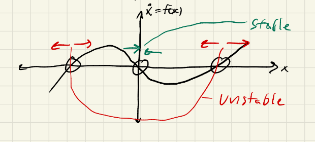
This implies
In higher dimensions \( \frac{\partial f}{\partial x} \text{is a Jacobian} \)
An eigen decomposition tells us if it is stable or not
Example: Pendulum Stability#
The system is unstable at \(\theta=\pi\) without control
import ForwardDiff as FD
using LinearAlgebra
u = 0
# At π
∂f∂x = FD.jacobian( x->dynamics(params, x, u), [π; 0])
eigvals(∂f∂x)
2-element Vector{Float64}:
 -9.904544411531505
  9.904544411531507
Pure imaginary values is called “marginally” stable
# At 0
∂f∂x = FD.jacobian( x->dynamics(params, x, u), [0; 0])
eigvals(∂f∂x)
2-element Vector{ComplexF64}:
 -0.0 - 9.904544411531507im
  0.0 + 9.904544411531507im
What about with our ideal control
# At π/2 with our ideal control
u = params.g*params.m*params.l
∂f∂x = FD.jacobian( x->dynamics(params, x, u), [π/2; 0])
eigvals(∂f∂x)
2-element Vector{ComplexF64}:
 -0.0 - 7.750414537183006e-8im
  0.0 + 7.750414537183006e-8im
# What about with our PD controller
X = [π/2; 0]
u = feedforward_pd(X, X, 3, 0.05)
∂f∂x = FD.jacobian( x->dynamics(params, x, u), X)
eigvals(∂f∂x)
2-element Vector{ComplexF64}:
 -0.0 - 7.750414537183006e-8im
  0.0 + 7.750414537183006e-8im
Adding damping will result in a strictly negative real part.